Here, the solidification is validated with the analytical solution known as the Neumann problem. The analytical solution to this solidification problem are used for example by Hu et al.[1] and Kawahara et al.[2].
Description of the Experiment
An initially liquid slab is cooled below its melting point from one side. The analytical solution for the temperature distribution and the position of the melt front is available for comparison with the simulation data. The interface position can be obtained from:
$$ x(t) =2Q \sqrt{\alpha t}~~~~~~(1)$$
Q is obtained from a transcendental equation that depends on the material properties and results to 1.19 for the material properties used in this comparison. α is the thermal diffusivity and t the time. The analytical solution for the temperature in the solid phase is
$$ T_s(x, t) = T_w + (T_m - T_w) * \frac{erf(x / (2.0 * \sqrt{\alpha_s *t)})} { erf(Q)}~~~~~~(2) $$
and for the liquid phase
$$ T_l(x, t) = T_{inf} + (T_m - T_{inf}) * \frac{erfc(x / (2.0 * \sqrt{\alpha_l * t}))} {erfc(Q)}~~~~~~(3)$$
The thermo physical properties are summarized in table.
| Parameter | Value |
|---|---|
| thermal conductivity | 400 W/(m*K) |
| density | 1000.0 kg/m³ |
| specific heat capacity | 1000.0 J/(kg*K) |
| latent heat | 200000.0 J/m³ |
| Tleft Wall | 173.15 K |
| Tright Wall | 283.15 K |
| Tmelt Initial | 283.15 K |
Description of Simulation Setup
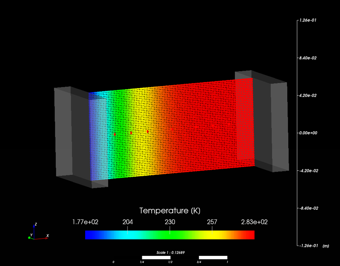
A two dimensional simulation is setup with one particle region for the melt and two polygonal regions for the left and right wall. The particle radius is set to 0.001 m and the influence of gravity is neglected. The geometric setup with the initial particle region is shown in figure below. Temperature samples are placed along the x-axis for comparison with the analytical result. The initial temperature of the liquid is set to 283.15 K. The left wall is set to a constant temperature of 173.15 K. This wall is used to cool down the initial liquid below its solidification point. The right wall is set to the same temperature as the initial fluid temperature.

Comparison of Simulation Results with Experiment
The simulation result of the temperature distribution at time point t = 4 s is shown in the figure below. The left and right walls are kept at their constant initial temperatures. The liquid is being cooled down from left to right.

The diagrams show a comparison between the analytical and simulation results at time t = 4 s. In the left diagram, the black line represents the analytical result for the solid temperature (see equation (2)), while the green line depicts the temperature distribution for the liquid phase (see equation (3)). The blue dots correspond to the simulated temperatures reported by the temperature samples. Overall, the analytical and simulated results exhibit good agreement.
The progression of the melt front is compared in the diagram on the right. The analytical result (black line) is calculated using equation (1), while the red dots represent the simulation results.


[1] H. Hu and S. A. Argyropoulos, “Mathematical modelling of solidification and melting: a review”, Modelling and Simulation in Materials Science and Engineering, vol. 4, no. 4, p. 371, 1996.
[2] T. Kawahara and Y. Oka, “Ex-vessel molten core solidification behavior by moving particle semi-implicit method”, Journal of Nuclear Science and Technology, vol. 49, no. 12, pp. 1156-1164, 2012.